Synchronization
A single machine has one clock and one shared memory, so ordering events and coordinating access to shared state is comparatively easy. A distributed system has neither: there is no global physical clock every node can read, no shared memory through which nodes can inspect each other, and any node or link may fail while the rest keep running. This chapter is about recovering, as far as possible, the coordination guarantees that a single clock would give for free. It proceeds from physical clock synchronization (keeping real clocks close), to logical time (agreeing on the order of events when exact time is unavailable), and then to the classic coordination problems that build on these foundations: mutual exclusion, leader election, global snapshots, termination detection, and distributed transactions with their concurrency control and deadlock machinery.
1. Synchronization in Distributed Systems#
Time matters in distributed applications for two broad reasons: executing an action at a given time, and timestamping data or messages so that event ordering can be reconstructed afterwards. The latter underpins file versioning, distributed debugging, and many security protocols. The recurring difficulty is that each machine timestamps events using its own local clock, and comparing timestamps across machines is only meaningful if those clocks agree.
1.1 Why Clock Synchronization Matters#
Having a perfectly synchronized clock across all nodes is equivalent to having a single global clock. Consider a shared file system where one machine runs an editor and another runs a compiler:
- The editor saves a source file at timestamp 21:43 (on the editor’s clock).
- The compiler compiles the object file at timestamp 21:44 (on the compiler’s clock).
In real (global) time the file was actually edited after the object was compiled. Comparing timestamps, the compiler concludes it does not need to recompile, because the object’s timestamp (21:44) looks later than the source’s (21:43). The conclusion is wrong, caused solely by the two clocks being out of sync. The lesson: when each machine timestamps events with its own local clock, cross-machine comparison is valid only if those clocks are synchronized.
1.2 What Is Time? Defining the Second#
The definition of the second has evolved:
- Astronomical time (until 1948). One second was defined as of the mean solar day (the average interval between successive solar noons, split into parts). The second was derived from the day. This is problematic because the Earth’s rotation is slowing, so the “day” gradually lengthens.
- Atomic time (TAI, since 1948). One second is defined as 9,192,631,770 oscillations of the cesium-133 atom, a number chosen to match the astronomical second as measured in 1948. This definition is constant and does not drift. TAI is collected and averaged in Paris from about 50 laboratories worldwide.
- UTC (Coordinated Universal Time). Reconciles atomic time with the slowing solar day by inserting a leap second whenever the skew grows large (threshold roughly 800 ms); about 30 leap seconds have been added since 1958. GMT is purely astronomical.
UTC is disseminated via radio stations (DCF77 in Europe, WWV in the US) and through GPS and GEOS satellites.
Because the Earth keeps slowing, the gap between atomic and astronomical time accumulates; when it exceeds about half a second a leap second is inserted. A well-known Google outage affected roughly half its data centers when some machines failed to apply a leap second: their clocks drifted out of sync, timestamp comparisons became inconsistent, and the distributed system crashed for several minutes. Time handling is not a detail.
1.3 Clock Drift and Synchronization Precision#
Every computer keeps time with a quartz-crystal oscillator, and even identical crystals oscillate at slightly different rates. This deviation is the clock drift rate, typically on the order of s/s, i.e. about 1 second every 11.6 days. Two quantities govern how often clocks must be resynchronized:
- Maximum clock drift rate : a hardware characteristic (how fast a clock departs from true time).
- Maximum allowed clock skew : an application requirement (the largest tolerable difference between two clocks).
If two clocks drift in opposite directions, over an interval they accumulate a skew of . To stay within they must be resynchronized at least every seconds.
Two flavours of requirement exist: some applications only need all clocks to agree with each other (internal synchronization), others need agreement with an external authoritative reference such as UTC. In all cases one rule is nearly universal:
Almost every protocol breaks if a clock jumps backward: events meant to be ordered can suddenly appear simultaneous or reversed. A clock that is found to be ahead must therefore never be set back. Instead it is slowed down (for instance, advanced 9 ms per tick instead of 10) until the others catch up. Freezing is possible but worse than slowing, because a frozen clock gives many events the same timestamp.
1.4 GPS-Based Synchronization#
GPS is the most accurate practical method. Satellites carry atomic clocks (mutually synchronized before launch), orbit at known positions, and broadcast messages carrying the timestamp of transmission. If a receiver had a perfect clock it could compute each signal’s travel time (reception minus send time), hence its distance to each satellite; two satellites (in 2D) or three (in 3D) would then fix its position.
In practice the receiver’s clock is not perfect, so its local time is treated as a fourth unknown. With four unknowns the receiver needs signals from four satellites and solves for position and its own clock offset simultaneously.
The GPS equations
Let be the unknown deviation of the receiver’s clock from the satellites’ atomic time, the receiver’s unknown coordinates, and the timestamp the -th satellite stamps on its message. If that message is received at receiver-time , the real reception time is , so, equating the measured distance with the true geometric distance and folding the clock error into :
Four satellites give four equations in the four unknowns , recovering both position and clock skew.
Cheap receivers achieve roughly 10 m spatial precision, corresponding to a few nanoseconds of time precision ( ns). The dominant error is usually the internal delay between the GPS chip and the system clock, not the algorithm. The limitations are cost and the need for line-of-sight to the sky, so GPS does not work inside buildings or data centers. This yields a natural hierarchy of time sources: a directly connected atomic clock (most accurate), then a GPS receiver, then network protocols such as NTP that synchronize against machines in the first two categories.
2. Synchronizing Physical Clocks#
GPS offers the best accuracy but needs dedicated hardware and a clear view of the sky. When that is unavailable, clocks are synchronized through message exchange. Three protocols do exactly that: Cristian’s algorithm, the Berkeley algorithm, and NTP.
2.1 Cristian’s Algorithm#
One designated time server holds the reference clock; every client synchronizes against it. The protocol is simply: the client asks the server for the time, the server reads its clock and replies, and the client adopts the value. Naively adopting the received value is imprecise, because time elapses while the reply travels back. The fix uses the round-trip time measured entirely on the client’s own clock, so its absolute drift cancels:
where is when the request was sent and when the reply arrived. The idea is that, on average, the server read its clock at the midpoint of the round trip, so adding half the RTT compensates for the reply’s flight.
Refinements
If the server reports the interval it spent handling the request, the estimate sharpens to , and the result is averaged over several measurements. Corrections are applied gradually (slowing or speeding the clock) so time never jumps backwards.
The correction is accurate only if the request and reply take approximately equal time in each direction and server processing is negligible. If the path is asymmetric, the server actually read its clock closer to one end of the round trip than the midpoint, and adding half the RTT over- or under-corrects. In general Cristian’s error is proportional to the asymmetry of the network path.
2.2 Berkeley Algorithm#
Cristian’s algorithm needs one machine with a trusted, correct clock. The Berkeley algorithm (from Berkeley Unix) removes that assumption: rather than tracking an authoritative source, it makes all clocks agree with each other, converging on a common time that need not be “real.”
- A time daemon periodically polls every machine for its current time.
- Each machine replies with its local time.
- The daemon averages all reported times (including its own), accounting for transmission delays.
- The daemon sends each machine the signed delta to apply.
For example, if the daemon reads 3:00, machine A reports 2:50 (10 min behind) and machine B reports 3:25 (25 min ahead), the average is about 3:05, so the daemon tells A to add 15 min, B to subtract 20 min, and itself to add 5 min. As with every protocol, a machine told to move backward must slow its clock rather than jump, so that no two events collapse onto the same timestamp.
2.3 Network Time Protocol (NTP)#
NTP is the current Internet standard for clock synchronization, pre-installed on essentially every operating system and designed to scale to billions of machines.
Machines are organized into layered strata: stratum 0 is a machine connected directly to an atomic clock; stratum 1 synchronizes against stratum 0; stratum 2 against stratum 1; and so on down to leaf end-user machines. Each node synchronizes with one or more nodes in the stratum above (its NTP server), configured manually or handed out by DHCP alongside the IP and DNS settings.
NTP facts
NTP runs over UDP, using multicast on a LAN and request/reply exchanges over the Internet, and has an estimated 10-20 million clients and servers. Reported accuracy is about 1 ms over LANs and 1-50 ms over the Internet. Stratum-1 servers connect directly to a UTC source, and stratum membership changes over time (more at www.ntp.org).
The way synchronization happens vary based on where the protocol is being used. On a LAN, the server can simply broadcast the time periodically, and receivers adopt it directly, assuming LAN delays are negligible for the target precision. Across the Internet, NTP uses a two-message exchange that also yields a bound on the error. Let A send to B and B reply to A, recording four timestamps:
- : A sends (A’s clock)
- : B receives (B’s clock)
- : B sends (B’s clock)
- : A receives (A’s clock)
Message carries all four values back to A. Now let’s call:
- : transmission time of , unknown
- : transmission time of , unknown
- : clock offset of B relative to A (what we want to estimate)
so, from the timing relationship:
We can define the round trip time as where it’s clear that the offset cancels out, so:
that is computable by A.\ Now let’s try to compute , where should not cancel out:
we can observe that the offset is composed by a computable part: , and an uncomputable part: , it can’t be computed since we don’t know the exact values of and .
We know, though, that the difference can’t be larger that the round trip time (), so we can say:
So the true offset is approximated by the computable , with error at most . A sends multiple message pairs to B. For each exchange, it computes (the estimated offset) and (the round-trip time, which bounds the error). NTP repeats the exchange and selects the exchange with the smallest , on the reasoning that the sample with the shortest round-trip is the one least affected by queuing delays and therefore the most reliable estimate of .
2.4 Practical Precision#
| Method | Typical precision | Notes |
|---|---|---|
| GPS | nanoseconds | Best possible; needs hardware and sky view |
| Atomic clock (direct) | nanoseconds | Most accurate; used at NTP roots |
| NTP on a LAN | ms | Sufficient for most local applications |
| NTP over the Internet | 10-50 ms | May be too coarse for fine event ordering |
For everyday uses (knowing when a class ends) Internet NTP is plenty. But when timestamps are used to order events that can occur milliseconds apart, a 10-50 ms skew may be unacceptable, and a GPS or local atomic reference is required. The rule of thumb: the tighter the required skew, the closer, in network terms, the time source must be.
3. Logical Time: Scalar (Lamport) Clocks#
Physical clocks can only be synchronized to within a bounded skew, and for many applications that is more than we need. Often it is enough to agree on the order of events rather than their exact time, which is the idea behind logical clocks.
3.1 Order Over Time#
Physical synchronization tells us how much time separated two events. But many applications only care whether one event happened before another. We do not care whether a file was edited one second or one day after the last compilation, only that it was edited after. A third party watching a question and its answer only needs the question to precede the answer; what would be harmful is seeing the answer first. What matters is order and causality, not precise timestamps. And if two processes never interact, directly or through a third party, their clocks may drift freely, because their events can never causally affect each other.
3.2 Lamport’s Happens-Before Relation#
These observations led Leslie Lamport, in a landmark 1978 paper, to the happens-before relation. An event is any action relevant to the application occurring within a process. This includes application-specific actions (reading a file, writing to disk, updating state) and, critically, two types of events that are always relevant in a distributed system sending: a message and receiving a message. Happens-before, written , is defined by three rules:
- Same process: if and occur at the same process and precedes locally, then .
- Message passing: if is the send of a message and is its receive, then .
- Transitivity: if and , then .
If neither nor , the events are concurrent, written .
Lamport argued that happens-before is the best available approximation of causality. Receiving a message is necessarily caused by its sending; an earlier event at a process may have influenced a later one; and processes that never exchange messages cannot have caused one another. The approximation is not perfect: it captures only potential causality over the channels the system can observe. In a chat application, sending someone a message just before they leave suggests your message caused it, yet they might have left because of a phone call, a channel invisible to the system. So means could have caused ; means could not have influenced through any observable channel.
3.3 Lamport Logical Clocks#
Lamport also gave a mechanism assigning each event a number that respects happens-before. Each process keeps a logical clock , initialized to 0:
- On any local event: increment by 1.
- Before sending: increment by 1 and attach it to the message.
- On receiving a message with timestamp : .
The construction guarantees one direction of an equivalence between clock order and causal order:
If then .
The proof follows the three rules: within a process the clock strictly increases; on message passing the receiver computes , strictly above the sender’s value; transitivity follows from transitivity of strict inequality. The converse does not hold. Two concurrent events can have different (even comparable) clock values without any causal link: if event on has value 1 and concurrent event on has value 2, then although . Formally,
3.4 Ordering Events#
Ordering all events by Lamport value therefore respects happens-before: whenever one event happened before another, it comes earlier in the ordering. But the ordering over-orders: it also imposes an order on concurrent events that happens-before leaves free. This is harmless, merely more conservative than necessary; sorting a deck by suit and number certainly sorts it by number too.
Happens-before is a partial order. Lamport values alone are also only a partial order, because two events at different processes may share a value. Appending the process id as a fractional part (process 1 starts at , process 2 at , and so on) makes every value distinct, yielding a total order that still respects happens-before while assigning an arbitrary but consistent order to concurrent events. A practical use is message reordering: a node that buffers incoming messages and processes them in Lamport order is guaranteed to handle a question before any reply to it, because answering necessarily follows receiving the question.
4. Totally Ordered Multicast#
Suppose a bank keeps two replicas of an account and two independent operations arrive: a customer deposits $100 (balance starts at $1000), and the bank applies 1% year-end interest. The two events are concurrent, neither caused the other, yet the final balance depends on their order.
This is the totally ordered multicast problem (also atomic multicast or atomic broadcast): every group member must deliver all messages in the same total order, even when the messages are causally independent.
4.1 Protocol (Assuming Reliable FIFO Channels)#
We assume the links are reliable (no message loss) and FIFO (messages arrive in send order on a given link). The protocol uses Lamport scalar clocks with fractional process ids for a strict total order:
- Multicast with timestamp. To multicast a message, a process sends it to all group members (including itself), stamped with its current Lamport clock.
- Queue on receipt. Each receiver puts incoming messages in a local queue ordered by timestamp, without delivering to the application yet.
- Acknowledge by broadcast. On receiving a message, each process broadcasts an acknowledgement to all members.
- Deliver when safe. A process delivers a message only when it is at the head of the queue (lowest timestamp) and acknowledgements from all other processes have arrived.
4.2 Why the Acknowledgements Are Necessary#
Holding a high-timestamp message at the queue head does not make it safe to deliver: a lower-timestamp message might still be in transit from another process. Waiting for every acknowledgement removes this ambiguity. Because channels are FIFO, receiving process ’s acknowledgement of guarantees that everything sent before that acknowledgement has already arrived, so no lower-timestamp message from can still be on the way. Once the message is at the head and all acknowledgements are in, no lower-timestamp message can ever arrive, and delivery is safe.
Concretely, suppose sends (timestamp 1) and sends (timestamp 2), and receiver has and all its acknowledgements. Could deliver before ? No: sent , then received , then acknowledged ; on the FIFO channel , precedes that acknowledgement, so if has the acknowledgement it already has , sitting ahead of in the queue and blocking it.
4.3 Cost#
For one message multicast to receivers, the sender transmits copies and each of the receivers broadcasts acknowledgements, giving messages per original message. Total ordering is expensive, which motivates the cheaper causal alternative below.
4.4 When Total Order Is Overkill#
Total order is often stronger than needed. In a group chat, two users who each send a message without seeing the other’s are concurrent; recipients only need to see them in the same order, and for many applications even that is unnecessary. The root issue is again the one-way implication whose converse fails: ordering by scalar clock inevitably orders concurrent events too. What we would ideally want is a timestamp with a co-implication,
so that numerical order is equivalent to causal order. Vector clocks achieve exactly this.
5. Vector Clocks and Causal Delivery#
Scalar clocks impose a total order stronger than causality requires. Vector clocks capture happens-before exactly, and enable a cheaper alternative to totally ordered multicast.
5.1 Vector Clocks#
Each process among keeps a vector clock , an array of integers. Position is ’s own event count (its scalar clock); position for is how many events at that is currently aware of, learned only by receiving messages (directly or indirectly). It is a distributed, partial view of the global state. The rules generalize the Lamport rule:
- Initialize all positions to 0.
- On a local event at : increment .
- Before sending at : increment and attach the whole vector.
- On receiving timestamp at : set for all , then increment to record the receive.
Vectors are compared component-wise:
- Equal:
- Less then or equal to:
- Strictly less than:
- Concurrent (parallel): ‒ there exists some position where is greater and another where is greater.
This is a partial order, and it matches happens-before in both directions:
By inspecting two timestamps alone we can now decide with certainty whether the events are causally related or concurrent.
5.2 Worked Example#
Tracing three processes from : has a local event , then sends, ; receives , merging and incrementing to , then sends, ; independently has a local event , then receives , giving . Checking the property: confirms ; and are incomparable, confirming ; and confirms .
Three processes end a run reporting , , . This is impossible. Position of any vector counts events at , and a process can never know of more events at than has itself recorded: . Here but , so claims to have seen 4 events at while produced only 3. Contradiction. (The same test rejects : .)
5.3 Causal Delivery#
For applications where only causality matters, causal delivery (deliver messages only in an order consistent with happens-before) is enough, and it is cheaper than totally ordered multicast. The protocol uses a simplified vector clock incremented only on sending, with no application-layer acknowledgements.
- On sending at : increment , attach , broadcast.
- On receiving a message with timestamp from sender at : deliver to the application iff both hold:
- : this is the next expected message from (none skipped);
- for all : the sender had seen no event that has not already delivered.
If a condition fails, the message waits in a queue; every delivery updates the clock (component-wise max) and re-examines the queue, so a held message may become deliverable. Condition 1 forbids gaps from the sender; condition 2 forbids delivering a message before something it causally depends on. For instance, if broadcasts with and receives it while holding , condition 2 fails (): had seen an event at that has not, so waits for that earlier message from before delivering ’s.
Is FIFO required?
Tanenbaum states that FIFO channels are required, but they are not. Condition 1 () already rejects an out-of-order message from and holds it in the queue until the gap fills, so FIFO is enforced by the protocol itself. Only reliable channels and broadcast are strictly needed.
| Property | Totally ordered multicast | Causal delivery |
|---|---|---|
| Clock type | Scalar (Lamport) | Vector |
| Acknowledgements | Broadcast ACKs required | None |
| Message complexity | per message | per message |
| Guarantee | Total order everywhere | Causal order only |
| Concurrent messages | Same order everywhere | May differ per receiver |
Causal delivery is simpler and cheaper but weaker; it is the right choice for chat-like systems where causally related messages must stay in order but the relative order of independent messages is irrelevant. (The global-state diagrams used here are illustrative: no single process ever sees this complete view; each acts on its local vector clock alone.)
6. Mutual Exclusion#
With a notion of event ordering in hand, we can tackle the classic coordination problems that are trivial with a shared clock but need real protocols without one. The first is mutual exclusion.
Mutual exclusion ensures that at most one process at a time holds a shared resource or executes a critical section. A centralized system solves this with hardware atomic instructions and mutexes built on a single clock; a distributed system has no such clock and needs dedicated protocols. Three properties are sought:
- Safety: at most one process holds the resource at a time (the core correctness requirement).
- Liveness: every request eventually succeeds; the system never deadlocks. Note the tension: blocking everything trivially gives safety but no liveness; blocking nothing gives liveness but no safety.
- Fairness (optional): if request happens-before request , access is granted to first.
All three protocols below assume reliable channels, and, unless stated, reliable processes.
6.1 Centralized Coordinator#
A single coordinator serializes access. A process asks the coordinator; if the resource is free it grants immediately, otherwise it queues the request and grants it when the current holder releases. (Equivalently, it may hand out a token that the holder returns when done.) This satisfies safety (the coordinator serializes everything), liveness (queued requests are eventually served), and fairness (by timestamping requests with logical clocks). It costs only 3 messages per access cycle (request, grant, release) and is the most message-efficient of the three. Its weakness is the single point of failure, though it is worth noting that the distributed alternatives fail if any process crashes, so one well-managed coordinator can be more robust in practice than potential failure points.
6.2 Ricart-Agrawala (Fully Distributed)#
There is no coordinator; processes decide collectively using Lamport timestamps. A process wanting the resource multicasts REQUEST(timestamp, P) to all others. A recipient responds by its state:
- Not interested: send
ACKimmediately. - Holding the resource: queue the request, reply later on release.
- Also waiting (has an outstanding request): compare timestamps. If ’s own request is earlier, queue ’s; if later, send
ACKnow (deferring to ). Ties break by process id.
enters the critical section once it has ACKs from all others, and on finishing sends the deferred ACKs to every queued requester. Safety holds because two processes could both enter only if each acknowledged the other, but the comparison rule forces one to queue the other. Liveness and fairness follow from granting priority to the lower timestamp, which approximates happens-before. The cost is messages per access cycle, and any single crash can block the system.
6.3 Token Ring#
The processes form a logical ring ordered by id, and a single token circulates continuously from each process to its successor. A process that does not want the resource forwards the token immediately; one that does waits for the token, holds it while using the resource, then passes it on. Safety holds because only the single token’s holder may enter; liveness holds because the token keeps circulating. Fairness is not guaranteed: a process may announce its intent just as the token passes it, letting an upstream neighbour that requested later acquire the resource first, because token-ring order is independent of happens-before order. The token also wastes bandwidth circulating when nobody wants the resource, and any crash breaks the ring, requiring repair.
6.4 Comparison#
| Centralized | Ricart-Agrawala | Token ring | |
|---|---|---|---|
| Safety / Liveness | ✓ / ✓ | ✓ / ✓ | ✓ / ✓ |
| Fairness (happens-before) | ✓ (with timestamps) | ✓ | ✗ |
| Messages per access | 3 | 1 to | |
| Delay before entry (msg times) | 2 | 0 to | |
| Points of failure | 1 (coordinator) | any process | any process |
The centralized solution is the most efficient and simplest, its cost being a single point of failure; the distributed alternatives instead have a distributed point of failure, since any crash can block everyone. Ricart-Agrawala is elegant and guarantees fairness at higher message cost; the token ring is simple and safe but unfair and wasteful when the resource is idle.
7. Leader Election#
Several protocols above rely on a single coordinator. When it fails, the survivors must agree on a replacement, the leader-election problem.
Algorithms such as centralized mutual exclusion or the initial token generator in a ring need exactly one distinguished process. If it crashes, the survivors must elect a new one: all non-crashed processes must agree on which process becomes coordinator.
7.1 Assumptions#
Processes carry unique identifiers (without them there is no basis for agreement); by convention the highest id wins, though the choice is arbitrary. The system is closed: every process knows the full set of ids, but not who is currently alive, which is what the election resolves. Crucially, crash detection requires synchrony. Detecting a crash uses either ping/pong or heartbeats, and both need a bound on transmission time, otherwise a slow message is indistinguishable from a crash. That in turn bounds network delay, clock skew, and processing time, i.e. a synchronous system. In a fully asynchronous system, reliable crash detection is impossible, so these algorithms simply assume synchrony.
7.2 Bully Algorithm#
When a process detects the leader has crashed, it starts an election toward higher ids; the highest live id “bullies” the rest into submission.
- Initiation: sends
ELECTIONto all processes with a higher id. - On receiving
ELECTION: a higher-id process repliesOK(taking over) and starts its own election upward. - Winning: a process that gets no
OKwithin a timeout declares itself leader and broadcastsCOORDINATOR. - Mid-election crash: a process that received
OKbut no subsequentCOORDINATORwithin a timeout assumes the would-be leader also crashed and restarts.
Multiple processes may start elections at once; they proceed in parallel and all converge on the same highest live id. Safety: the highest live id wins. Liveness: with reliable, synchronous channels (so timeouts are meaningful) the election terminates. If the network partitions, each side elects its own leader, and whether two leaders are acceptable depends on the application. In the worst case (process 0 initiates) messages are exchanged.
7.3 Ring-Based Election#
Processes form a logical ring ordered by id; each knows its successor. The ring is logical, requiring only that any process can contact any other.
- Initiation: on detecting the crash, a process sends an
ELECTIONmessage carrying its own id to its closest live successor (skipping crashed nodes). - Forwarding: each recipient appends its own id and forwards to its next live successor.
- Termination: when the initiator receives its own id back, the message has toured the ring and lists all live ids; the initiator picks the highest and sends a
LEADERmessage around the ring.
Concurrent elections are handled because each process forwards every election message but acts only when its own token completes the circuit; all tokens collect the same live set and elect the same process. If the elected process crashes mid-announcement, conflicting LEADER messages are resolved by checking which candidate is actually alive. Safety: all completing processes agree on the leader. Liveness: while the ring survives, the election terminates. Fairness is not guaranteed (ring order is not happens-before order). Cost is per circuit (one ELECTION round, one LEADER round), or with concurrent initiators.
| Bully | Ring | |
|---|---|---|
| Message complexity | worst case | per round |
| Concurrent elections | handled | handled |
| Mid-election crashes | timeout + restart | token verification |
| Result | highest live id | highest live id |
| Synchrony | required | required |
Both need every node reachable by every other (the ring is a logical abstraction) and both need synchrony for crash detection. The bully algorithm is simpler to reason about but more expensive; the ring is cheaper but must manage the ring structure and successor failures.
8. Collecting Global State and Distributed Snapshots#
Beyond coordinating individual actions, we sometimes need a coherent picture of the whole system at once, for checkpointing, recovery, or checking global invariants. Capturing such a state without a shared clock is the distributed-snapshot problem.
8.1 Why Collect Global State?#
An application’s state is inherently distributed: each node holds its local state, and the totality of these plus the messages in transit defines the global state. The primary motivations for collecting global state include:
- Fault tolerance: if a crash occurs, restarting from a saved global state (a checkpoint) is far better than starting over. Ideally everyone would freeze at the exact same instant, but in a real system messages fly fast and states change quickly, so an instantaneous global picture is effectively impossible.
- Invariant Checking: Global snapshots can verify that critical global properties hold. For instance, in a distributed banking system, the total amount of money, including all node balances and any money currently in transit, must be rigorously preserved.
8.2 The Banking Example#
Consider banks transferring money among themselves, with money neither created nor destroyed (a constant total, say 120 units, spread across balances and in-transit transfers). A snapshot must preserve the total, which includes both balances and money in transit. The classic error: bank A saves its state before sending a transfer, while bank B saves after receiving it. The snapshot then shows the money at B while A’s balance was never reduced, inflating the total, an inconsistent, invalid state.
8.3 Consistent vs Inconsistent Cuts#
A cut is a picture of the system formed by freezing each process at a (possibly different) point, , where is ’s event history up to its cut point.
A cut is consistent iff, for every event , every event with is also in :
Equivalently: if a message receive is in the cut, its send must be too. The converse need not hold, a message may be sent but not yet received (in transit). A cut that includes receiving at but not sending at is inconsistent: it records a receive with no matching send, which cannot happen. A cut that includes the send but not the receive is consistent: is simply in transit, and sliding CPU/channel speeds yields a real configuration matching it.
8.4 The Chandy-Lamport Algorithm#
The Chandy-Lamport distributed snapshot is among the most widely used protocols in the field: it collects a consistent global snapshot without halting the application. Its assumptions are reliable links and nodes (extensible), a strongly connected graph (every node reachable from every other), and FIFO channels.
Any process may initiate a snapshot (no election needed). To start, a process performs three steps atomically (guarded by a brief local lock): record its own state; send a marker (token) on every outgoing channel; begin recording all incoming channels. When a process receives a marker for the first time, it likewise atomically records its state, sends markers on all outgoing channels, and begins recording every incoming channel except the one the marker arrived on (that channel is immediately closed, recorded as empty). When later receives a marker on a channel it is already recording, it stops recording that channel; the messages recorded there are exactly those that were in transit across the cut. A process’s snapshot is complete when it has received a marker on every incoming channel; strong connectivity guarantees this eventually happens everywhere.
The protocol is non-blocking: only the brief atomic initialization interrupts a process. When a message arrives on a channel being recorded, the process records it and also processes it normally, so the application is never meaningfully paused.
Every message is accounted for exactly once in the snapshot: it is either reflected in the recorded state of a process (received before that process saved) or recorded as in transit on exactly one channel (it crossed the cut), never both and never neither. Post-snapshot messages (sent after the sender saved and received after the receiver saved) belong to neither and simply fall outside the snapshot.
This invariant is the practical key to solving snapshot exercises: track each message and decide whether it lands in a node’s saved state, on a channel, or entirely after the cut.
8.5 Worked Example#
Take a process with two incoming channels and one outgoing channel.
| Step | Event | Action |
|---|---|---|
| 1 | marker on | save state; close (empty); send marker out; start recording |
| 2 | message on the closed channel | process normally; do not record |
| 3-4 | messages on | record each and process normally |
| 5 | marker on | close ; ’s snapshot complete |
contributes: its state as saved at step 1; ; and (the messages in transit when the cut was taken).
8.6 Correctness#
The algorithm records a consistent cut
Let at processes . It suffices to show (the definition of a consistent cut). Suppose instead is recorded but is not; then occurred before saved, while occurred after saved.
If , then precedes in one history, so recording records , contradiction. Otherwise across processes means a message chain . Since came after saved, sent its marker before , hence before : the marker is ahead of . Since came before saved and the marker triggers that save, the marker reached after . So the marker started ahead of the chain yet arrived behind it: it was overtaken. This is impossible under FIFO channels (a marker cannot be passed on a channel by a later message) and atomic marker forwarding (a process forwards markers before processing any later incoming message, so nothing jumps ahead at an intermediate node). Contradiction.
In-transit messages recorded on channels are replayed into their receivers on restart, so recovery is lossless; for the correctness proof they may be set aside, as sent-but-not-received messages do not violate consistency.
8.7 Extensions#
The base protocol admits several variants: a blocking variant halts computation and buffers channels (simpler, more disruptive); snapshot collection forwards each local snapshot to a collector that assembles the global state; incremental snapshots record only changes since the last one, making frequent snapshotting practical; and concurrent snapshots run several instances in parallel, each marker tagged with a unique snapshot id so a channel may be recording for several ids at once without interference. Beyond recovery, snapshots support invariant checking: periodically collecting a global state and verifying, for instance, that total money (balances plus in-transit) is conserved, all without stopping the system.
9. Termination Detection#
One important use of a global snapshot is to determine whether a distributed computation has actually finished, a surprisingly subtle question, since a system can look idle while a message is still in transit.
A distributed computation has terminated only when all processes are idle and all channels are empty. The second condition is the subtle one: every process may be idle at some instant while a message still travels a channel and will reactivate a process on arrival. Neither the sender (already moved on) nor the receiver (not yet in) knows about that in-transit message, which makes termination a genuinely distributed problem.
9.1 Via a Distributed Snapshot#
The direct solution is to run Chandy-Lamport and inspect the result: if every process recorded itself idle and every channel state is empty, the computation has terminated. The drawback is cost: the full snapshot must be collected on one node, transmitting every process and channel state.
9.2 A Flawed Lightweight Proposal#
Tanenbaum’s textbook proposes a lighter-weight alternative that reuses the structure of the Chandy–Lamport protocol without storing the full snapshot. The idea is to propagate markers as before, but instead of recording messages, each process only tracks whether it received any message during the protocol, and reports a DONE or CONTINUE message back toward the initiator:
- The predecessor of a process is the process from which received its first marker.
- The successors of are all processes to which forwarded the marker.
- When has received markers from all its incoming channels, it sends a
DONEmessage to its predecessor only if all three conditions hold:- P has finished its application work.
- P received no application messages between receiving its first marker and receiving its last marker.
- All of P’s successors have already sent DONE to P.
- Otherwise, P sends CONTINUE.
- If the initiator receives DONE from all its successors, the computation is declared finished. Otherwise, a new snapshot is triggered.
The flaw lies in the definition of successor. When forwards the marker to all its outgoing channels, not all of those recipients necessarily receive ’s marker as their first marker. One of them may have already received a marker from a different process, making that other process their predecessor, not . As a result, waits for DONE replies from processes that will never send a DONE message (because they report to a different predecessor). P waits indefinitely. The protocol deadlocks.
The fix is to tighten “successor” to mean a process actually activated (whose first marker came from ), which is exactly what the next algorithm does.
9.3 Dijkstra-Scholten#
This applies to diffusing computations: processes are idle by default, activate only on receiving a message, and the whole computation starts from a single external event that activates one process, which activates others, and so on. The algorithm maintains an activation spanning tree:
- The process that got the original request is the root.
- When active sends a message that activates an idle , an edge is added: is ’s parent.
- When sends to an already active , immediately replies “do not count me as your child”; no edge is added.
A process reports completion to its parent once it is idle and all its children have reported. When the root is idle with all children reported, the computation is terminated. The tree grows (new activations) and shrinks (completed subtrees) dynamically; a finished process may be reactivated and rejoin as a new child. Using a tree (not a DAG) gives each process exactly one parent to report to, removing the ambiguity that broke Tanenbaum’s proposal.
| Approach | Correct | Cost | Applicability |
|---|---|---|---|
| Chandy-Lamport snapshot | ✓ | high (full state) | general |
| Tanenbaum’s protocol | ✗ | n/a | : |
| Dijkstra-Scholten | ✓ | lower (control messages) | diffusing computations |
The Tanenbaum proposal is a useful cautionary tale: conflating “processes I sent a marker to” with “processes I activated” breaks the protocol entirely. Distributed algorithms are easy to get almost right and hard to get exactly right.
10. Distributed Transactions and Concurrency Control#
We now move from coordinating events to coordinating data. Distributed transactions extend the familiar ACID guarantees across multiple nodes.
A transaction is a sequence of reads and writes on a data store that must satisfy ACID: Atomicity (all-or-nothing), Consistency (valid state to valid state), Isolation (concurrent transactions do not interfere), and Durability (committed effects survive failures). A transaction is delimited by begin and either commit or abort. This chapter targets full ACID compliance, which is markedly harder in a distributed setting where data may be partitioned or replicated across nodes.
Distributed transactions come in two forms. Nested transactions form a hierarchy: a top-level transaction spawns sub-transactions (each on a private copy of its data, typically on a different host), and durability applies only to the top level, a committed sub-transaction is undone if its parent aborts. Flat transactions have a single begin/commit/abort boundary but may touch data on many nodes; they look flat to the programmer while the system coordinates behind the scenes. The flat case is the focus here.
10.1 Atomicity: Private Workspaces vs Write-Ahead Logs#
Atomicity is implemented in two main ways. With a private workspace, a transaction works on a private copy of the data it touches: the index is copied in at the start, all reads and writes hit the copy, commit atomically swaps the private index for the original (a fast in-memory pointer swap), and abort just discards the workspace. This is optimistic about commits (commit is a swap; abort is even cheaper).
With a write-ahead log (WAL), the transaction modifies the database in place but first records each change (transaction id, item, old value, new value) in a persistent log. Commit is trivial (data already in place); abort replays the log in reverse, restoring old values. This is pessimistic about aborts (abort does work; commit is instant). For example, running x = x+1; y = y+2; x = y*y from logs [x:0/1], [y:0/2], [x:1/4]; on abort these are replayed in reverse to restore .
| Private workspace | Write-ahead log | |
|---|---|---|
| Commit cost | low (index swap) | very low (already in place) |
| Abort cost | very low (discard) | higher (reverse replay) |
| Best when | aborts expected | commits expected |
10.2 Isolation and Serializability#
Isolation’s formal criterion is serializability: a concurrent (interleaved) execution is serializable if it produces the same result as some serial execution of the same transactions (each running start-to-finish with no interleaving). There is no single correct order; matching any serial order suffices. For three transactions on a shared (, , ) the serial orders yield , so an interleaving leaving matches no serial order and is not serializable. Matching a serial final value is necessary but not, in general, sufficient, serializability is properly judged on the order of conflicting operations. Only read-write and write-write pairs conflict; read-read does not. The concurrency controller’s job is to allow as much parallelism as possible while permitting only serializable interleavings, along two design axes: locks vs explicit ordering, and pessimistic vs optimistic.
A distributed database typically has a Transaction Manager (lifecycle: begin/commit/abort), Schedulers (decide operation order, enforce serializability), and per-site Data Managers (physically read/write, via workspaces or logs). If data is partitioned, each site’s scheduler owns its data; if replicated, schedulers holding replicas must coordinate. Coordination options for replicated data are: elect a master copy (all access through the master scheduler, simple, but a bottleneck/SPOF), distributed locking (acquire locks across replicas), or timestamp ordering (order operations by transaction timestamp rather than locks).
The two concurrency-control families are locking (pessimistic: acquire a shared read lock or exclusive write lock before access, wait if unavailable, release on commit/abort, risks deadlock) and timestamp ordering (each transaction gets a timestamp at creation; operations must respect timestamp order or the offending transaction is aborted and restarted, no locks, but aborts on violation, best under low contention).
11. Locking and Timestamp Ordering#
The two families introduced above are examined in detail here, including their distributed variants.
11.1 Two-Phase Locking (2PL)#
A transaction must lock an item before accessing it, under one rule:
Once a transaction releases any lock, it may never acquire another.
This splits execution into a growing phase (acquire locks, possibly interleaved with reads/writes) and a shrinking phase (release locks, no new acquisitions), which never overlap. The rule provably makes every 2PL execution equivalent to a serial one. Strict 2PL goes further, releasing all locks only at commit/abort; collapsing the shrinking phase to the end prevents cascading aborts (no transaction reads uncommitted data) and is the variant most used in practice.
Distributed 2PL has three variants:
- centralized: a single lock manager node handles all lock requests for the entire system. Simple to reason about, but a bottleneck and single point of failure;
- primary-copy: each data item has one designated master replica. The scheduler at the master node is responsible for granting locks on that item, regardless of which replica is actually being accessed. A transaction accessing a local copy must still contact the master scheduler to obtain the lock;
- fully distributed: each site has its own scheduler, responsible for data stored locally. Schedulers coordinate with each other to ensure that a lock granted at one site does not conflict with a lock held at another. This requires a synchronization protocol among schedulers and is the most complex variant.
2PL guarantees serializability but does not prevent deadlock: holds item 1 and waits for item 2 while holds item 2 and waits for item 1, and the cycle may span more transactions. Deadlocks must be detected and resolved (Section 12).
11.2 Pessimistic Timestamp Ordering#
Instead of locks, each transaction gets a unique timestamp at creation (typically a Lamport clock, tying order to an happens-before relationship). Each data item tracks two values:
- : the timestamp of the latest transaction that read ;
- : the timestamp of the most recent committed transaction that wrote .
Write operations are not applied immediately. Instead, they are stored as tentative versions, each tagged with the writing transaction’s timestamp. Multiple tentative versions may coexist. A tentative version becomes the committed version when its transaction commits; it is discarded if the transaction aborts.
A write by is accepted as a new tentative version iff
Intuitively:
- If : a newer transaction has already read the value. Accepting ’s write would retroactively change what that newer transaction read, a violation of serializability. is aborted.
- If : a newer transaction has already committed a write. is trying to write an obsolete value that has already been superseded. is aborted.
A read by is accepted only in 3 cases, first the scheduler finds the latest version of whose timestamp is less than or equal to , let’s call this version . Three cases arise:
- Case 1: is the committed version and : The read is satisfied immediately. Return the value of and update .
- Case 2: is a tentative version: The scheduler cannot yet know whether will commit (in which case its value is correct) or abort (in which case the previous committed value should be returned). The read request is suspended (placed in a wait queue) until the transaction that wrote either commits or aborts. Once that outcome is known, the scheduler resumes the read.
- Case 3: (the committed version is newer than ): The committed value reflects a transaction newer than . The scheduler no longer has the value that held at time . The read request has arrived too late. is aborted.
| Request | Condition | Action |
|---|---|---|
| Write by | and | accept as tentative |
| Write by | either fails | abort |
| Read by | selected version committed | return immediately |
| Read by | selected version tentative | wait |
| Read by | abort |
Crucially, pessimistic timestamp ordering never deadlocks: the only waiting is a read waiting for one specific tentative write to resolve, which always terminates (commit serves the read; abort removes the version and the read is served from the next eligible one). There is no circular dependency. An aborted transaction restarts with a new, higher timestamp, gaining priority next time.
11.3 Optimistic Timestamp Ordering#
In a large database with many small transactions, the chance that two concurrent transactions touch the same item is often tiny. Both 2PL and pessimistic ordering do work up front for conflicts that rarely materialize; the optimistic approach bets conflicts are rare and checks almost nothing during execution. Transactions run freely on a private workspace (or log), and at commit the scheduler validates that no item they read or wrote was modified by another transaction since they started (by comparing timestamps). If validation passes, commit; if a conflict is found, abort and restart (cheap, since changes were private). It gives maximum parallelism and is deadlock-free, but under heavy load it triggers many rollbacks, which is why it is not widely used, especially in distributed systems.
| Property | 2PL | Pessimistic TS | Optimistic TS |
|---|---|---|---|
| Deadlock possible | ✓ | ✗ | ✗ |
| Transactions abort | ✗ (wait) | ✓ (at access) | ✓ (at commit) |
| Conflict detected | at access | at access | at commit |
| Best under | moderate contention | moderate contention | low contention |
The essential difference between the two timestamp schemes is when conflicts are detected: pessimistic ordering aborts immediately on an out-of-order request, limiting wasted work; optimistic ordering discovers conflicts only at commit, so under high contention a transaction may do much work only to be rolled back.
12. Detecting and Preventing Distributed Deadlocks#
Locking buys serializability at the risk of deadlock. This final topic covers detecting deadlocks after they form and preventing them from forming at all.
Deadlock is a cycle of waiting: holds and waits for , holds and waits for , possibly extended to . There are four strategies: ignore (assume deadlocks are astronomically rare), detect and recover (let them happen, then break the cycle), prevent (make deadlock structurally impossible), and avoid (prove at runtime no path leads to deadlock, rarely used in distributed systems). We focus on detection/recovery and prevention. A helpful fact: in transactional settings, recovering by aborting and rolling back a transaction is far less disruptive than killing a process, which makes transactions a convenient framework for handling deadlocks.
12.1 Detection and Recovery#
Detection means finding a cycle in the wait-for graph (an edge meaning waits for a resource held by ). Centrally this is easy; distributed, the graph is spread across nodes with only local views, and no instantaneous global picture exists, so a cycle may be reported that has already dissolved, or a real one missed.
A coordinator that assembles per-node wait-for graphs (updated on every arc change, periodically, or on demand) can perceive a cycle that never existed, because reports arrive at different times. If releases and then acquires , but the coordinator processes one host’s update before another’s, it may momentarily “see” a cycle and needlessly abort a transaction. This motivates the coordinator-free probe below.
The probe-based algorithm (Chandy-Misra-Haas, 1983) avoids a global snapshot. When a process has waited past a timeout, it sends a probe carrying (initiator, sender, receiver) to the process holding the resource it wants. A blocked recipient appends itself and forwards the probe to whoever holds its wanted resource; a non-blocked recipient drops it (no cycle on that path). If the probe returns to its initiator, a cycle is confirmed.
To break the cycle, one process is aborted (releasing its resources): the initiator itself, or the highest-id, lowest-id, or cheapest-to-restart process. In databases, deadlocks are rare and small, roughly 90% of cycles involve just two processes [Gray, 1981], so the simplest policy is for the initiator to abort itself; to avoid many initiators aborting redundantly, a common alternative is to abort the highest-id process in the cycle (which is why each process appends its id to the probe).
12.2 Prevention: Timestamp-Based Schemes#
Prevention makes cycles structurally impossible by giving each transaction a global timestamp at creation and imposing a consistent direction on all wait-for edges, so the wait-for graph is always a DAG. A cycle would require waiting “backward” in timestamp order at some point, which both schemes forbid.
Wait-die. When wants a resource held by : if is older (lower timestamp) it waits; if is younger it aborts itself (“dies”) and retries later with a new (higher) timestamp. All waiting edges point from older to younger, so no backward edge, hence no cycle. Old transactions wait; young ones die and retry.
Wound-wait. When wants a resource held by : if is older it preempts (“wounds”) , forcibly aborting it, and proceeds; if is younger it waits. All waiting edges point from younger to older, so again no cycle. Old transactions run uninterrupted; young ones may be preempted repeatedly (each restart gives a higher timestamp, keeping them young), until the older conflicting transaction completes.
| Wait-die | Wound-wait | |
|---|---|---|
| Old wants young’s resource | old waits | old preempts young |
| Young wants old’s resource | young dies | young waits |
| Aborts fall on | young | young (via preemption) |
| Abort frequency | higher | lower |
| Deadlock possible | never | never |
Wound-wait typically causes fewer aborts, because a young transaction is preempted only when an older one actively needs its resource, whereas in wait-die a young transaction dies immediately whenever it would have to wait for an older one. In both, the wait-for graph stays acyclic, so deadlock cannot occur by construction.
| Approach | Deadlock | Overhead | Applicability |
|---|---|---|---|
| Ignore | ✓ | none | only if deadlocks are astronomically rare |
| Detect + recover (probe) | ✓ then resolved | probes on timeout | general |
| Prevent via snapshot | ✗ | full snapshot cost | general but expensive |
| Wait-die | ✗ | more aborts | distributed transactions |
| Wound-wait | ✗ | fewer aborts | distributed transactions |
13. Exam questions#
Cugola does not publish exam solutions. The worked answers below are unofficial: our own reconstructions, following the conventions used in the course slides and the professor’s clarifications from the Q&A session. Use them as a study aid, not an authoritative key.
13.1 Clock synchronization#
Describe and compare the approaches to synchronize clocks in a distributed system. Then suppose you must correlate readings of geographically distributed vibration sensors to locate the origin of an earthquake with precision under 1 km (seismic waves travel at most 10 km/s). Which synchronization approach would you use, and why?
Solution
Comparison (see Sections 1-2). GPS / direct atomic clock: nanosecond precision, but needs hardware and, for GPS, sky view. Cristian’s algorithm: a client corrects for latency using half the round trip against a time server; error grows with path asymmetry. Berkeley: no authoritative clock, a daemon averages everyone’s time and hands out deltas (internal synchronization only). NTP: the Internet standard, a stratum hierarchy with a bounded-error two-message exchange; roughly 1 ms on a LAN, 10-50 ms over the Internet.
Seismic sensors. The epicenter is found by comparing arrival times across sensors, so a clock error translates into a position error of about . For under 1 km with km/s: The clocks must agree to well within 100 ms. Internet NTP (tens of ms, and the relative skew between two sensors can approach 100 ms) is borderline and risky. GPS is the right choice: the sensors are outdoors with a clear sky view, GPS gives nanosecond-level time (far below the 100 ms budget), and it also provides each sensor’s position for free, which the localization needs anyway.
Describe and compare the various approaches to synchronize node clocks in a distributed system.
Solution
A pure comparison question: the same four approaches as above (GPS/atomic, Cristian, Berkeley, NTP). A good answer states, for each, the mechanism, the precision, the assumptions, and the trade-offs, GPS best but hardware/sky-bound; Cristian simple but assumes symmetric latency and a trusted server; Berkeley needs no authoritative clock but only synchronizes internally; NTP scalable and self-installing with a computable error bound but coarser over the Internet. Close with the rule of thumb: the tighter the required skew, the closer the time source must be.
13.2 Scalar clocks and totally ordered multicast#
Describe how scalar clocks implement totally ordered multicast (state the assumptions). Compare with a solution based on a central server that receives messages over point-to-point links and dispatches them to every member over point-to-point links. Focus the comparison on traffic and the assumptions each protocol needs.
Solution
Scalar-clock protocol (Section 4). Stamp each multicast with a Lamport clock (fractional process id for a strict total order); every receiver queues messages by timestamp and broadcasts an acknowledgement to all; a message is delivered only when it is at the queue head and every other process has acknowledged it. Assumptions: reliable and FIFO channels, and (for liveness) no process crashes, since a missing acknowledgement blocks delivery. Traffic: one multicast costs message copies plus acknowledgements, i.e. per message.
Central server. The sender sends to the server (1 message); the server forwards to each of the members ( messages), so per message. The order is defined simply by the server’s arrival order over FIFO links, no clocks needed. Assumptions: reliable FIFO links to and from the server; the server is a single point of failure and a throughput bottleneck.
Comparison. The central server generates far less traffic ( vs ) and needs no logical clocks, but concentrates all load and failure risk in one node. The scalar-clock solution has no ordering bottleneck and no special node, at quadratic message cost and with the property that any crash blocks progress (all acknowledgements are required). The choice is the familiar centralized-vs-distributed trade-off.
Describe how scalar clocks implement a totally ordered multicast primitive, clarifying the assumptions required.
Solution
The protocol and assumptions of Section 4: Lamport timestamps with fractional ids, timestamp-ordered queues, broadcast acknowledgements, and the “head of queue and all acknowledgements received” delivery rule, over reliable FIFO channels. The FIFO assumption is what lets an acknowledgement stand in for “all earlier messages from this sender have already arrived,” which is the crux of correctness.
13.3 Mutual exclusion with scalar clocks#
Describe the mutual-exclusion problem and how to solve it with scalar clocks. Which properties does the protocol satisfy, and under which assumptions does it work?
Solution
This is the Ricart-Agrawala algorithm (Section 6.2). A process multicasts REQUEST(ts, id) with its Lamport timestamp; a recipient replies ACK at once if uninterested, queues silently if it holds the resource, and if it is also competing compares timestamps, deferring (queuing) to the lower one and acknowledging the higher (ties by id). A process enters the critical section after collecting ACKs from all others and, on exit, releases its queued deferrals. It satisfies safety (two entrants would each have acknowledged the other, impossible under the comparison rule), liveness (lowest-timestamp requests are granted immediately, and holders release), and fairness (priority by Lamport order approximates happens-before). Assumptions: reliable channels and reliable processes, a single crash withholds an ACK and blocks everyone. Cost is messages per access.
13.4 Vector clocks#
Write the vector-clock values for the situation in the figure, then briefly describe an algorithm that leverages vector clocks.
Solution
(The 2015 figure is not reproduced here; the method is identical to the worked example of Section 5.2, which we use as the model.) Apply the three rules, increment your own position on a local event or before sending, and on receipt take the component-wise max then increment your own position. For our example this gives , , , , , . A leveraging algorithm is causal-delivery multicast (Section 5.3): messages carry the sender’s send-incremented vector, and a receiver delivers only when the message is the next expected from its sender () and the sender had seen nothing the receiver has not ( for ), buffering otherwise. Vector clocks give the exact needed to enforce this.
13.5 Distributed snapshot with a spurious message#
The system in the figure is running a distributed snapshot; every process adds the value of each received message to its state . Process A started the snapshot, recording state 2 and sending tokens to B and E, which have already processed them and sent out their own tokens. Show the state captured by every node (local state and messages recorded per link), and state your assumptions. Note: there is one spurious message in the figure, identify and remove it before running the snapshot.
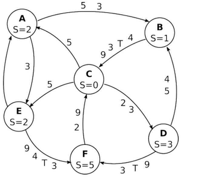
Solution
Step 1, find the spurious message. Application messages (plain numbers) cannot be judged spurious: any value is plausible. Only tokens obey a verifiable rule, a process may emit a token only after receiving its first token (or after initiating). So we check every token against its sender’s history:
- A initiated, so its tokens on and are legitimate (already consumed by B and E).
- B received A’s token, so B’s token on is legitimate.
- E received A’s token, so E’s tokens on and are legitimate.
- D emitted a token on , but D’s only incoming channel is , which carries no token (C has not saved state, so C sent no token). D never received a token, so its outgoing token cannot exist: it is the spurious message. Remove the token on (its application messages 3 and 9 stay).
Step 2, who has saved state. After removing the spurious token, the consistent picture is: A, B, E have saved (A initiated; B and E received A’s token). C, D, F have not yet saved, their incoming tokens are still in transit (, ) or absent.
Step 3, run to completion. Recall the invariant: each in-transit message ends up in exactly one place, folded into the receiver’s saved state (if received before it saved), recorded on one channel (if it crosses the cut), or entirely post-snapshot. Messages ahead of a token on the same channel arrive before that token, so they are forced; only cross-channel races need an assumption.
Assumption: on the two cross-channel races, the currently in-transit application messages arrive at their destination after that destination has saved, so they are recorded rather than folded in, specifically, the messages on and on are recorded. (The alternative timing, arrival before the save, folds them into C’s and F’s states and records empty channels; both are valid, and the assumption must be stated.)
Working it through:
- A (saved ). Records and (both arrive after A saved, before the closing tokens).
- B (saved ). is B’s first-token channel, recorded empty; the later 5,3 on it are post-snapshot. Records .
- E (saved ). is E’s first-token channel, recorded empty. Records .
- C. Its first token arrives on ; the 9 and 3 ahead of that token are delivered first, so C saves . is recorded empty; (by the assumption). C then emits tokens on .
- D. Its first (and only) token arrives on ; the 2 and 3 ahead of it are delivered first, so D saves . recorded empty. D emits tokens on and .
- F. Its first token arrives on ; the 9 and 4 ahead of it are delivered first, so F saves . recorded empty (the trailing 3 is post-snapshot); (by the assumption).
Captured snapshot.
| Node | Saved | Recorded incoming channels |
|---|---|---|
| A | 2 | , |
| B | 1 | , |
| C | 12 | , |
| D | 8 | |
| E | 2 | , |
| F | 18 | , |
Every in-transit message lands in exactly one place (a saved state, a recorded channel, or post-snapshot), which confirms consistency. The two starred messages ( and ) are the assumption-dependent ones: swapping the assumption moves them from their channels into C’s and F’s saved states instead.
Same setup, without the spurious-message twist: A starts, records its state, and sends tokens to B and E, which have already forwarded their own; show the captured state per node and state the assumptions.
Solution
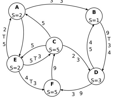
These use the same graph and method as above, minus the spurious-token step (no token violates the “emit only after receiving one” rule, so nothing is removed). Solve identically: (1) identify which nodes have already saved (A, plus every node that has received a token); (2) for each incoming channel, record what arrives after the receiver saves and before that channel’s token, and record empty on the channel a node’s first token arrived on; (3) fold into a node’s saved state the application messages it delivers before its own token; (4) state assumptions for any cross-channel timing races. The figure for the 12 Jul 2024 variant is reproduced below.
Variant: explicit channel-speed assumptions (1 Feb 2013 / 27 Jun 2013)
Older versions of this exercise (A records state 12) make the timing assumption explicit, for example “channels leaving B are much faster than the others, channels leaving E are very slow.” Such wording removes the ambiguity: it fixes the arrival order of the cross-channel messages, and hence which are folded into states versus recorded on channels. The lesson is exactly the one flagged above, when the arrival order is not determined, the exercise has several correct answers, so the assumption must always be declared.
13.6 Pessimistic timestamp ordering#
Describe pessimistic timestamp ordering: which problem does it address, and how does it work? In a system with few requests per second and a large dataset, would you use pessimistic or optimistic timestamp ordering, and why?
Solution
Problem. Enforce isolation/serializability among concurrent transactions without locks (hence without deadlock).
Mechanism (Section 11.2). Each transaction gets a unique timestamp at creation; each item tracks its last read timestamp and last committed write timestamp, and writes are held as tentative, timestamp-tagged versions. A write by is accepted only if exceeds both the item’s read and write timestamps, else aborts (it would invalidate a newer read or overwrite a newer write). A read returns the latest committed version ; it waits if that version is tentative, and aborts if a committed write newer than already exists (it arrived too late). Aborted transactions restart with a higher timestamp. No cycle of waiting can form, so there is no deadlock.
Few requests, large dataset. Low contention: two concurrent transactions almost never touch the same item, so conflicts are rare. Here optimistic ordering is preferable, it does essentially no checking during execution and validates only at commit, so in the common (conflict-free) case it pays almost no overhead, whereas pessimistic ordering checks timestamps on every access for conflicts that will rarely occur. Optimistic’s weakness (many rollbacks under heavy contention) does not bite when contention is low.
13.7 A note on leader election#
Leader election (bully and ring, Section 7) is standard examinable material, but it does not appear as a standalone written question in the exam set available to us. As a self-test, redo the worked figures: with the old leader crashed, trace the ELECTION/OK/COORDINATOR exchange of the bully algorithm and the id-collecting circuit of the ring algorithm, and confirm both elect the highest live id.
14. Glossary#
| Term | Meaning |
|---|---|
| Clock drift rate | Rate at which a hardware clock departs from true time (about s/s for quartz). |
| Clock skew | Difference between two clocks; the maximum tolerable value is an application requirement. |
| UTC / TAI / GMT | Civil atomic time with leap seconds / pure atomic time / purely astronomical time. |
| Cristian’s algorithm | Client synchronizes to a time server, correcting by half the measured round trip. |
| Berkeley algorithm | A daemon averages all clocks and distributes deltas; internal synchronization only. |
| NTP | Internet clock-sync standard; stratum hierarchy; two-message exchange with error bound . |
| Event | Any relevant action at a process, including message send and receive. |
| Happens-before () | Partial order capturing potential causality; concurrent if unrelated in both directions. |
| Lamport (scalar) clock | Integer counter; , but not the converse. |
| Vector clock | Per-process array; (both directions). |
| Totally ordered multicast | All members deliver all messages in one common order; with scalar clocks + ACKs. |
| Causal delivery | Deliver only in happens-before-consistent order; with vector clocks. |
| Mutual exclusion | At most one process in the critical section; centralized, Ricart-Agrawala, or token ring. |
| Leader election | Agree on a single coordinator (highest live id); bully or ring; needs synchrony. |
| Cut | Prefix of each process’s history; consistent if every recorded receive has its send recorded. |
| Marker (token) | Control message delimiting “before” and “after” the snapshot on each channel. |
| Chandy-Lamport | Non-blocking distributed snapshot capturing a consistent cut; needs FIFO, strong connectivity. |
| Diffusing computation | Computation started by one external event; basis for Dijkstra-Scholten termination detection. |
| ACID | Atomicity, Consistency, Isolation, Durability. |
| Serializability | A concurrent schedule equivalent to some serial one; the correctness criterion for isolation. |
| 2PL | Two-phase locking: no lock acquired after any release; strict 2PL releases all at commit. |
| Timestamp ordering | Order operations by transaction timestamp; pessimistic (abort at access) or optimistic (at commit). |
| Wait-for graph | Directed graph of “waits for” edges; a cycle is a deadlock. |
| Wait-die / wound-wait | Timestamp-based deadlock prevention keeping the wait-for graph acyclic. |